2006 USGS North Puget Sound LIDAR survey: Data quality

Ralph Haugerud
U.S. Geological Survey
c/o University of Washington
Seattle, WA
31 March 2008, updated 20 March 2009

The North Puget Sound lidar survey was an experiment in low-cost collection of lidar data over a large area. The USGS and the contractor learned a great deal from this experiment. The resulting data have already proven useful for certain earthquake hazards research tasks, some geomorphic and geologic mapping, and some flood-hazard analyses. However, the data do not meet Task Order specifications for completeness or accuracy.

Users of these data should be aware of several data quality issues which are summarized below.

Completeness

There are two small unsurveyed areas in the vicinity of the North Fork Nooksack River, one on the ridgecrest NE of Canyon Lake and another at the US-Canada border NE of Silver Lake.

There are three areas of sparse returns due to too-low return intensity (dropouts), a consequence of flying too high with insufficient laser power. These are along lower Finney Creek south of Concrete, near Marblemount along the Skagit River and Cascade River valleys and extending as far north as the confluence of Bacon Creek with the Skagit River, and along the Skagit River in the vicinity of Ross Dam.

Some collected data were omitted from the delivered data set. Lidar data are collected in swaths a few hundred meters wide and--typically--many kilometers long. Each swath corresponds to a single pass of the aircraft carrying the lidar instrument. Data from a single swath were segmented into tile fragments and tile fragments from multiple, overlapping swaths were then concatenated to produce tiles of multi-swath data. In the processing of this survey, many tile fragments were omitted. This is evidenced by abrupt changes in 1st-return density at tile boundaries. Examples are shown in the images below.

Click on images for larger versions

Shaded-relief images of highest-hit surface. Yellow = NODATA. Cyan lines are boundaries of 3,000 ft x 3,000 ft LAS data tiles. Black labels are LAS data file names.

Overall, that part of the NPS survey that was acquired with the Leica ALS-50 averages about 1.4 pulse/m². However, in the sidelap areas (about 50% of the area surveyed), points from one of the overlapping swaths were excluded from ground-point classification. The effect is a mean pulse density for this part of the survey of about 0.9 pulse/m². That part of the survey that was acquired with the Optech 2050 has a mean pulse density of 1.3 pulse/m². Several LAS tiles in this area (including PS3515, PS3939, PS4300, PS4468, PS4469, PS4470, PS4578, and PS4579) have pulse densities less than 0.5 pulse/m².

Spatially variable return classification

For almost all lidar surveys, identification of some lidar returns as "ground" is largely by automated computer routines, typically with classification parameters that are adjusted by a human analyst to obtain the best results. The results of automated return classification may then be reviewed and revised by a human analyst. While largely automated, these procedures of necessity have a subjective component. On large surveys, it is not uncommmon to find that the rules for return classification vary significantly from place to place.

Careful inspection will show that in some places significant numbers of vegetation or building returns are classified as ground; in other, similar, settings they are not. Automatic return classification procedures commonly fail to identify bluff edges as ground, and in places this is the case for this survey. In a few locales, negative blunders (points that are significantly too low) have not been identified as such, and corner-removing routines have identified the adjacent ground returns as not-ground, leaving distinctive "bomb craters" in the resulting bare-earth DEM.

Unusual characteristics of LAS files

For that part of the North Puget Sound area surveyed with the Leica ALS-50 instrument, large numbers of returns are identified as class 10. These class 10 returns appear to be limited to the margins of swaths in areas of overlap with adjoining swaths. Apparently, swaths were trimmed of sidelap (within area of overlap, all returns within one swath identified as class 10) then pieced together prior to classification of some returns as ground. According to the ASPRS LAS standard, class 10 is reserved for eventual later definition.

Areas surveyed with the Optech 2050 instrument, which records first and last returns only, are distinguishable in part because the associated LAS files have subequal numbers of 1st and 2nd returns. In many cases, LAS files record more 2nd returns than 1st returns. This does not make sense. What the return numbers mean and how this occurred are unknown.

Accuracy

At several locales in the eastern part of the survey, significant steps at swath boundaries give an impression of the likely vertical reproducibility of the survey measurements. A few of these are shown below.

Click on images for larger versions


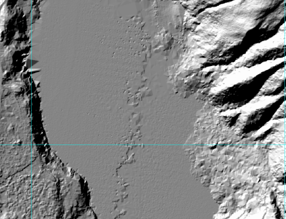
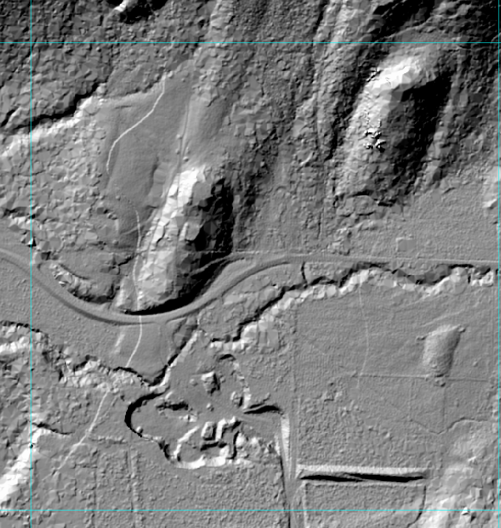
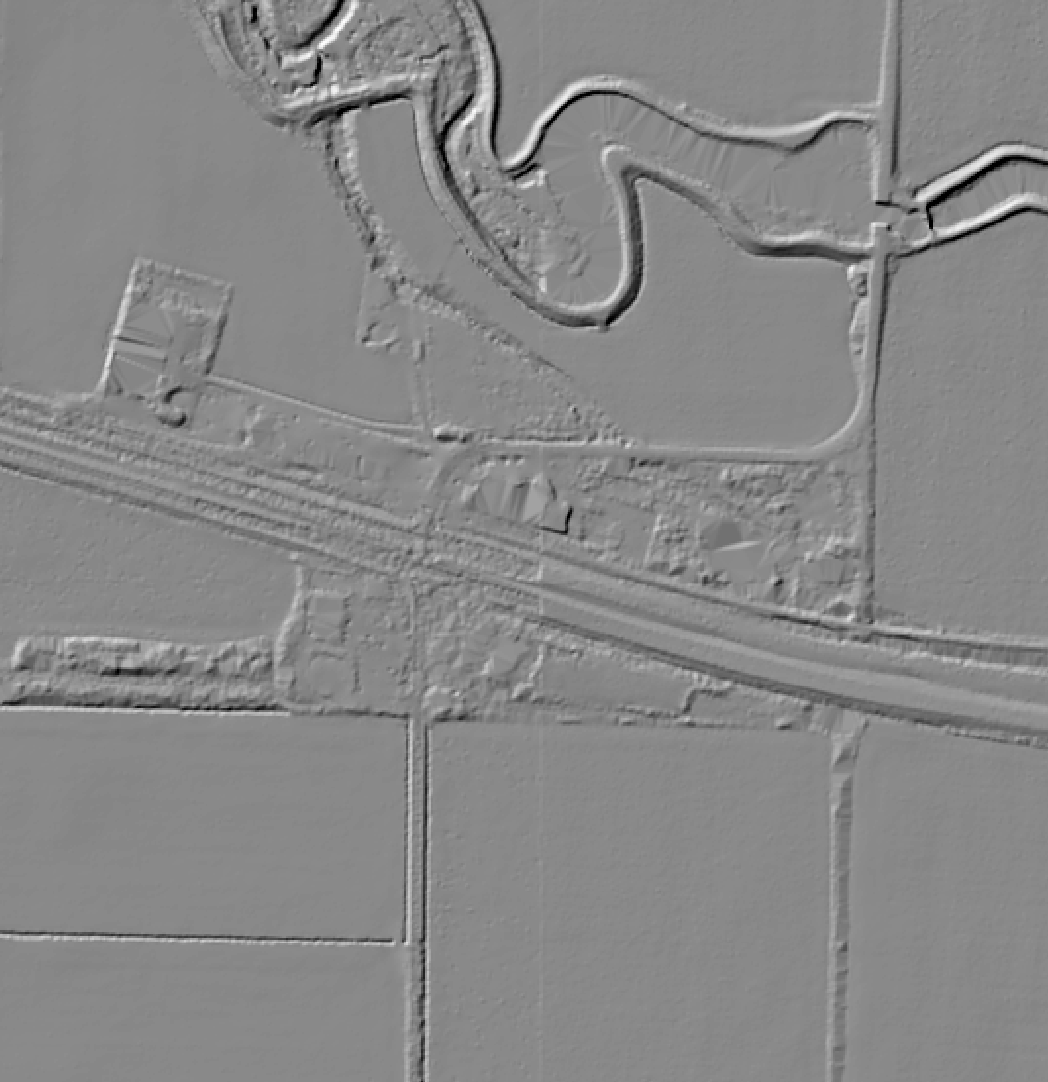
Swath-boundary step, Silver Lake, north of Maple Falls (N Fk Nooksack drainage). Swath boundary is irregular because of erratic specular reflection (no light returned to instrument) at margin of near-nadir zone. West side of lake is 2 1/2 ft higher than east side. Cyan lines are boundaries of 3,000 ft square LAS tiles.	Multiple swath-boundary steps in N Fk Nooksack valley east of Kendall. Swath boundaries are curvilinear because of aircraft roll. Where western step crosses highway in left-center part of image, step is 3 1/2 ft high. Cyan lines are boundaries of 3,000 ft square LAS tiles.	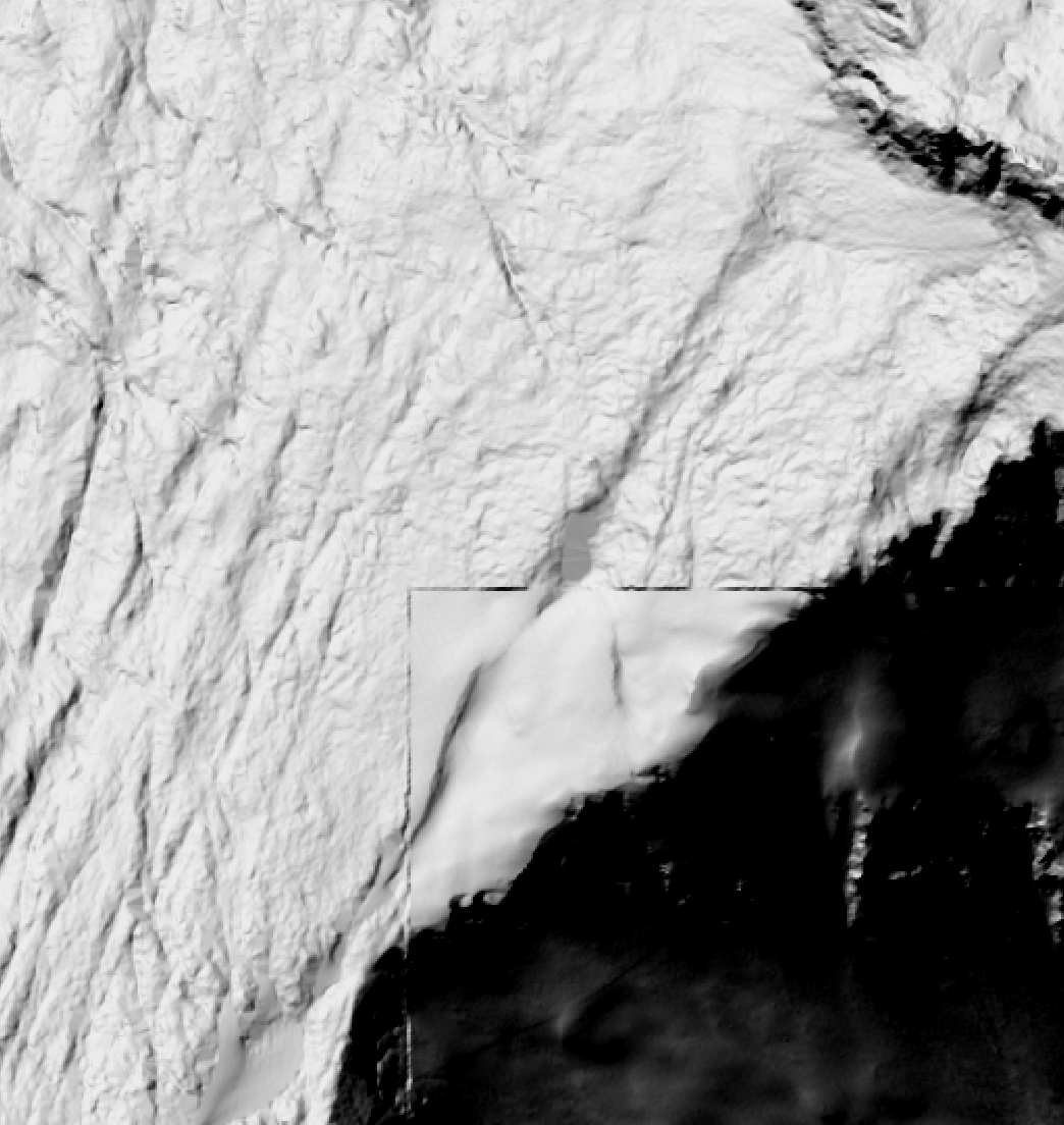Step at tile boundary on ridge crest southeast of Skagit River near Newhalem. Image is of area about 3,000 feet wide. Omission of some swath fragments has located swath-swath differences at tile boundaries. Vertical difference at the step is as large 10 feet. Note that area south of the step is smoother, probably because it was surveyed in early summer with significant snow cover, whereas higher side is more rugged as the snow had melted. True vertical difference between overlapping swaths must be significantly greater than 10 feet.

There are vertical steps at some tile boundaries, as well as variations in road-surface heights that suggest variable compensation for range walk (range walk is the variation of apparent height with reflectance, such that brighter targets appear closer to the lidar instrument). The steps at tile boundaries strongly suggest that swath fragments were adjusted vertically to minimize swath-swath mismatches within single tiles, at the expense of continuity between tiles.

Click on images for larger versions

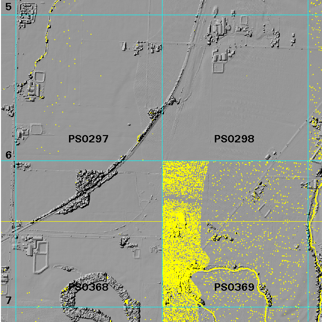
North-south vertical step at tile boundary, State Route 20 west of Burlington. Step is about 0.5 ft in fields to south of highway. Along highway, step is nearly 4 ft. Lumpy, too-low surface of western part of highway may reflect uncompensated range walk.

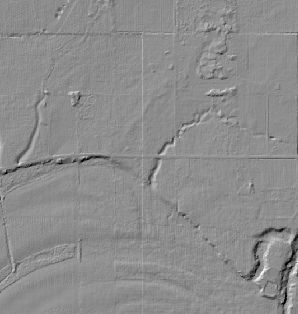
North-south vertical step at tile boundary, Skagit valley southeast of Sedro Woolley. Step is about 0.75 ft high at road in center of image.

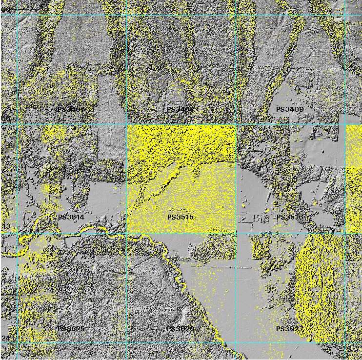
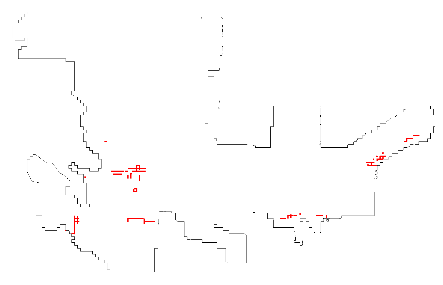
Outline of survey area with observed tile-boundary steps in red. Zipped ESRI .e00 file of observed tile-boundary steps; zipped shape file of observed tile-boundary steps. Note that this inventory of tile-boundary steps is almost certainly incomplete.

Quantitative analysis of the swath to swath consistency of lidar measurements indicates that, for the region surveyed with the Leica ALS-50, RMS Z reproducibility is circa 10 cm and RMS XY reproducibility is circa 83 cm. There is significant evidence that the error distribution is abnormal, perhaps because of vertical adjustment of swath fragments within some tiles to minimize misfits. I think it is likely that the true RMS Z reproducibility of this part of the survey is significantly different, perhaps on the order of 15 cm.

For the region surveyed with the Optech 2050, RMS Z reproducibility appears to be 20 cm and RMS XY reproducibility appears to be circa 96 cm. Again, the error distribution is abnormal, thus it is not clear that these numbers truly reflect the reproducibility of the survey.

Background colors on the diagrams below indicate data density. Contours enclose 99%, 95%, 90%, 75%, 50%, 25%, and 10% of data. 95 and 50 percentile contours are red. Heavy black lines are RMS y for each value of x. White lines are weighted least-squares best-fit quadratic.
Click on images for close-ups of areas near (0,0)

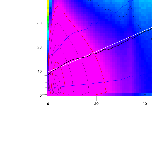
Local slope - swath difference diagram for "west" part of NPS survey (that area surveyed with the Leica ALS-50). Note overabundance of local slope = 0, abs(DELTA Z) = 0 values (click on image to see close-up). True RMSE Z difference may be as high as 15 cm.

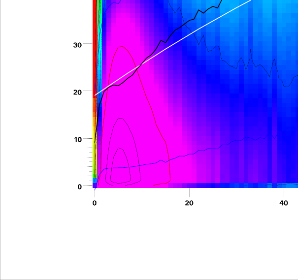
Local slope - swath difference diagram for "east" part of NPS survey (that area surveyed with Optech 2050). Complex, convex-up shape of best-fit line suggests this is not a single population of swath differences and thus the P1 (RMSE Z difference) and P2 (RMSE XY difference) values obtained from this analysis are likely incorrect.

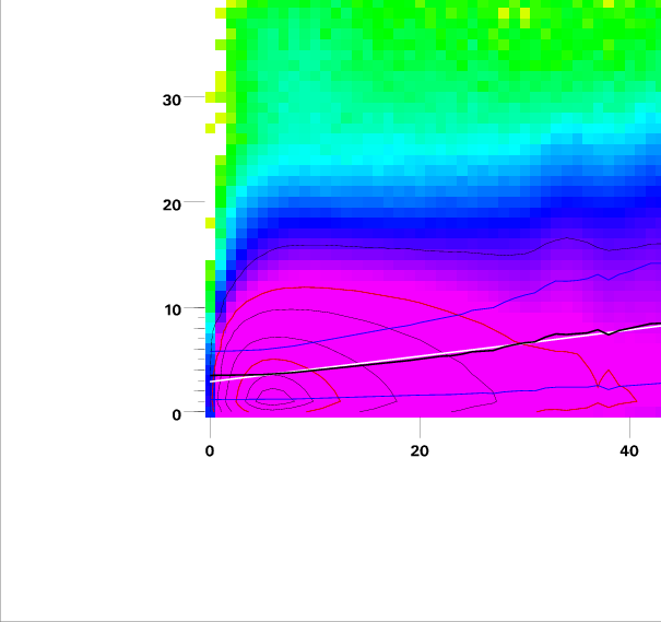
Local slope-swath difference diagram for 2007 Puget Sound Lidar Consortium survey in vicinity of Portland, Oregon. Diagram suggests a well-behaved single population of swath differences, with P1 (RMSE Z difference) = 2.9 cm, P2 (RMSE XY difference) = 25 cm.

Experience with many lidar surveys in this rugged, heavily forested region suggests that the internal reproducibility of bare-earth DEMs is usually on the order of 1.5 to 2 times poorer than the reproducility of raw lidar measurements. This is borne out by analysis of this survey, where internal reproducibility of the interpolated ground surface is on the order of 1 foot (west area, Leica ALS-50) or 2 feet (east area, Optech 2050).

Note that in all cases the observed swath to swath consistency places a lower bound on the absolute accuracy of the survey, as there may be long-wavelength errors that are not captured by the consistency analysis.

In the Report of Survey (.doc version), (.pdf version), the contractor reports that 60 checkpoints were surveyed by GPS, and that

"Although 60 points where collected, the resulting LiDAR terrain in areas of 15 points proved unaccepted for proper statistical analysis in these areas resulting in the dismissal of these points."

The remaining 45 checkpoints data indicate a root mean square Z error (RMSE Z) of 0.554 ft.